Tutorial 6 Modeling activity patterns with covariates
Many researchers exploring activity patterns from camera-trap data sooner or later run into the challenge of estimating how activity patterns vary in response to some conditions, often related to the environment in which the data have been collected. We address this common set of ecological questions in this Tutorial, focusing first on categorical and then on continuous variables.
6.1 Categorical covariates
The task of comparing activity patterns among different levels of a categorical variable can be achieved using KDE approaches. However, the process can be particularly cumbersome, especially when comparing more than two levels. It requires splitting the dataset of the independent records depending on the levels of the variable of interest, run a KDE for each group of records, and then comparing the results using an ad-hoc test. Conversely, the same task can be accomplished by fitting a hierarchical model to the whole dataset, as we describe here. In Tutorial 9.4, we repeat this same analyses using the KDE approach, and compare results to those obtained using the trigonometric and cyclic cubic spline hierarchical models.
Again, we use camera-trap records collected between 2016 and 2018 at 100 locations in Northern Minnesota, USA (Iannarilli et al. 2021). This time, we use records of American black bear (Ursus americanus) and explore differences in activity patterns of this species between spring and fall.
# Load Libraries
rm(list = ls())
set.seed(129)
library(dplyr)
library(lubridate)
library(GLMMadaptive)
library(mgcv)
library(ggpubr)
library(forcats)
# Load data
dat <- read.csv("data_input/species_records.csv") %>%
filter(Species == "BlackBear") %>% droplevels() %>%
mutate(DateTimeOriginal = ymd_hm(DateTimeOriginal))
cov <- read.csv("data_input/CameraTrapProject_CT_data_for_analysis_MASTER.csv", as.is = TRUE) %>%
mutate(Date_setup = mdy(Date_setup),
Date_retr = mdy(Date_retr),
Problem1_from = mdy(Problem1_from),
Problem1_to = mdy(Problem1_to)
)
# Extract Season information from Session column
dat$Season <- as.factor(substr(dat$Session, 1, 1))
# Merge time of deployment and retrieval + problems
site <- cov
site$end <- ymd("2000-01-01")
for(i in 1:nrow(site)){
site$end[i] <- min(site$Date_retr[i],
site$Problem1_from[i],
na.rm = TRUE
)
}
# Create dataframe to store captures
occasions <- vector("list", length = nrow(site))
for(i in 1:nrow(site)){
occasions[[i]] <- data.frame(Session = site$Session[i],
Site = site$Site[i],
start = seq(from = ymd_hms(paste(site$Date_setup[i], "00:00:00", sep = " ")),
to = ymd_hms(paste(site$end[i], "23:59:59", sep = " ")), by = '60 min'
)
) %>%
mutate(end = c(start[2:length(start)],
start[length(start)]+minutes(60)
)
)
}
occasions <- do.call(rbind.data.frame, occasions)
occasions$capt <- 0
# Store captures
for(i in 1:nrow(dat)){
occasions[occasions$Session == as.character(dat$Session[i]) & occasions$Site == as.character(dat$Station[i]) &
occasions$start <= dat$DateTimeOriginal[i] & occasions$end > dat$DateTimeOriginal[i], "capt"] <- 1
}
# Format data
occasions$Time <- hour(occasions$start)
occasions$Season <- as.factor(substr(occasions$Session, 1, 1))
table(occasions$Season, occasions$capt)##
## 0 1
## F 222236 244
## S 347923 773We obtained 773 (out of 348 696) and 244 (out of 222 480) hourly occasions with at least 1 positive record of a bear in the Spring and Fall sessions, respectively.
We again format the data using a cbind(success, failure) structure as described in Tutorial 4, but this time we also create an additional column (Season) that contains the information about the season (i.e. Spring or Fall) in which the records were collected and use it as an additional grouping criterion.
occasions$Site <- as.factor(occasions$Site)

# format data for cbind(success, failure)
occasions_cbind <- occasions %>%
  group_by(Site, Time, Season) %>%
  summarize(success = sum(capt),
            failure = n() - success)
## `summarise()` has grouped output by 'Site', 'Time'. You can override using the `.groups` argument.## # A tibble: 6 × 5
## # Groups: Site, Time [3]
## Site Time Season success failure
## <fct> <int> <fct> <dbl> <dbl>
## 1 10A 0 F 0 100
## 2 10A 0 S 0 159
## 3 10A 1 F 0 100
## 4 10A 1 S 0 159
## 5 10A 2 F 0 100
## 6 10A 2 S 0 159We save this dataset for applications in other parts of the tutorial.
6.1.1 Trigonometric GLMMs
Extending the trigonometric hierarchical models to explore the effect of a covariate on activity patterns only requires the inclusion of interactions between the trigonometric terms and the covariate. The interactions allow the coefficients of the trigonometric terms to vary by treatment group, in this case, the two levels of the covariate Season. We start by fitting and visualizing estimated activity curves for the two seasons based on a random intercept-only model in which the random intercept for Site accounts for repeated measures and varying levels of activity at each site:
# run model
trig_rand_int <- mixed_model(fixed = cbind(success, failure) ~
                                              cos(2 * pi * Time/24) * Season +
                                              sin(2 * pi * Time/24) * Season +
                                              sin(2 * pi * Time/12) * Season +
                                              cos(2 * pi * Time/12) * Season,
                             random = ~  1  |   Site,
                             data = occasions_cbind,
                             family = binomial(),
                             iter_EM = 0
                             )
summary(trig_rand_int)
##
## Call:
## mixed_model(fixed = cbind(success, failure) ~ cos(2 * pi * Time/24) *
## Season + sin(2 * pi * Time/24) * Season + sin(2 * pi * Time/12) *
## Season + cos(2 * pi * Time/12) * Season, random = ~1 | Site,
## data = occasions_cbind, family = binomial(), iter_EM = 0)
##
## Data Descriptives:
## Number of Observations: 4800
## Number of Groups: 100
##
## Model:
## family: binomial
## link: logit
##
## Fit statistics:
## log.Lik AIC BIC
## -2284.197 4590.394 4619.051
##
## Random effects covariance matrix:
## StdDev
## (Intercept) 0.9022139
##
## Fixed effects:
## Estimate Std.Err z-value p-value
## (Intercept) -7.3343 0.1216 -60.3133 < 1e-04
## cos(2 * pi * Time/24) 0.4808 0.1102 4.3629 < 1e-04
## SeasonS 0.7450 0.0869 8.5698 < 1e-04
## sin(2 * pi * Time/24) -0.5554 0.0989 -5.6164 < 1e-04
## sin(2 * pi * Time/12) -0.1697 0.0980 -1.7311 0.0834365
## cos(2 * pi * Time/12) -0.2358 0.0986 -2.3904 0.0168278
## cos(2 * pi * Time/24):SeasonS -0.7353 0.1275 -5.7657 < 1e-04
## SeasonS:sin(2 * pi * Time/24) 0.3460 0.1100 3.1453 0.0016592
## SeasonS:sin(2 * pi * Time/12) -0.4507 0.1131 -3.9863 < 1e-04
## SeasonS:cos(2 * pi * Time/12) -0.3739 0.1135 -3.2945 0.0009859
##
## Integration:
## method: adaptive Gauss-Hermite quadrature rule
## quadrature points: 11
##
## Optimization:
## method: quasi-Newton
## converged: TRUE# build estimate of activity
newdat <- with(occasions_cbind,
expand.grid(Time = seq(min(Time), 24, length.out = 48),
Season = levels(Season)
)
)
pred_rand_int <- effectPlotData(trig_rand_int, newdat, marginal = FALSE) # plot
(pl_trig <- ggplot(pred_rand_int, aes(Time, plogis(pred))) +
geom_ribbon(aes(ymin = plogis(low), ymax = plogis(upp), color = Season, fill = Season), alpha = 0.3, linewidth = 0.25) +
geom_line(aes(color = Season), linewidth = 1) +
scale_color_manual(values = c("orange", "darkgreen")) +
scale_fill_manual(values = c("orange", "darkgreen")) +
coord_cartesian(ylim = c(0, 0.005)) +
labs(x = "Time of Day (Hour)", y = "Predicted Activity Pattern \n (probability)", title = "A: Hierarchical model, Trigonometric GLMM \n(random intercept-only)")+
theme_minimal()+
theme(legend.position = "bottom",
legend.title = element_blank(),
legend.text = element_text(size=10,face="bold"),
legend.margin=margin(0,0,0,0),
legend.box.margin=margin(-5,-10,-10,-10),
plot.title = element_text(size=10,face="bold"),
axis.line = element_line(colour = 'black', linetype = 'solid'),
axis.ticks = element_line(colour = 'black', linetype = 'solid'),
axis.title = element_text(size=9,face="bold"),
panel.grid.minor.y = element_blank(),
panel.grid.major.y = element_blank(),
panel.grid.major.x = element_line(colour = 'lightgrey', linetype = 'dashed', linewidth=0.5),
panel.grid.minor.x = element_blank(),
strip.text = element_text(size = 9, colour = "black", face = "bold", hjust = 0)
) +
scale_x_continuous(breaks=seq(0,23,length.out=7), labels=seq(0,24,4))
) 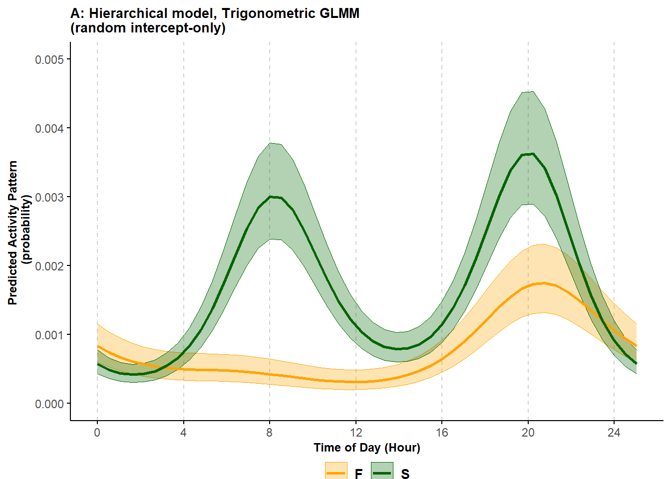
Figure 6.1: Predicted probability of activity of black bears in the spring (S) and fall (F) using a random intercept-only trigonometric hierarchical model; shading corresponds to 95% confidence intervals.
The estimated activity patterns show a striking difference between the two seasons. In Spring, black bears had a bimodal activity pattern, with the species active primarily around around 8:00 and 20:00. During the Fall, the species was mostly inactive during the morning.
Importantly, the two seasons were sampled for a different number of days since the study included 3 springs but only 2 falls. This difference in sampling effort makes the direct comparison between the intensity of activity in the two seasons difficult when using KDEs. However, both the trigonometric GLMMs and the cyclic cubic HGAMs (see later) directly account for sampling effort and make this comparison possible. Thus, we can also say that the probability of a black bear being active around 20:00 was overall higher in the Spring than in the Fall.
Model selection: To test the importance of the seasonal effect on activity patterns of black bears, we can also compare the model above with a model that does not include the covariate using AIC:
# run model
trig_rand_int_no_cov <- mixed_model(fixed = cbind(success, failure) ~
                                              cos(2 * pi * Time/24) +
                                              sin(2 * pi * Time/24) +
                                              sin(2 * pi * Time/12) +
                                              cos(2 * pi * Time/12),
                                    random = ~  1  |   Site,
                                    data = occasions_cbind,
                                    family = binomial(),
                                    iter_EM = 0
                                    )
AIC(trig_rand_int, trig_rand_int_no_cov)
## df AIC
## trig_rand_int 11 4590.394
## trig_rand_int_no_cov 6 4774.190The AIC comparison supports the model that includes a seasonal effect on bears’ activity patterns.
We could consider further extending the interaction model by including random slopes.
trig_rand_slope <- mixed_model(fixed = cbind(success, failure) ~
                                              cos(2 * pi * Time/24) * Season +
                                              sin(2 * pi * Time/24) * Season +
                                              sin(2 * pi * Time/12) * Season +
                                              cos(2 * pi * Time/12) * Season,
                               random = ~  cos(2 * pi * Time/24) * Season +
                                           sin(2 * pi * Time/24) * Season +
                                           sin(2 * pi * Time/12) * Season +
                                           cos(2 * pi * Time/12) * Season  ||   Site,
                               data = occasions_cbind,
                               family = binomial(),
                               iter_EM = 0
                               )
summary(trig_rand_slope)
However, this model is likely to be too computational demanding for most laptops. In such cases, we can either opt for the simpler model - keeping in mind that we are not allowing the estimates to vary in their timing of activity - or we can run this model on a computing cluster.
6.1.2 Cyclic cubic spline HGAMs
Similar to trigonometric GLMMs, cyclic cubic spline HGAMs can also be used to model activity patterns as a function of a categorical covariate. As we explained in Tutorial 3, this class of models is highly flexible and offers a plethora of options when it comes to choosing a model structure. Here we focus on two model specifications. The first resembles a trigonometric random intercept-only GLMM and contains Season as a fixed term, a cubic cyclic smoother for Time which varies by Season, and a smoother for Site as a random effect. This structure accommodates variability in the frequency of site-use, but not in the timing of activity.
# 'Random intercept-only'
mod_cycl1 <- bam(cbind(success, failure) ~
                   Season +
                   s(Time, bs = "cc", k = 12, by = Season, m = 1) +
                   s(Site, bs="re"),
                  knots = list(Time=c(0,23)),
                  family = "binomial",
                  data = occasions_cbind
                 )

# Predict activity patterns
newdat <- with(occasions_cbind,
               expand.grid(Time = seq(min(Time), max(Time), 1),
                           Season = levels(Season),
                           Site = "7B" #Station doesn't matter
                           )
               )


cycl_pred1 <- predict.bam(mod_cycl1,
                          newdata = newdat,
                          exclude = "s(Site)",
                          se.fit = TRUE,
                          type = "response"
                          )
cycl_pred1 <- cbind(newdat,
                    fit=cycl_pred1$fit,
                    se.fit=cycl_pred1$se.fit,
                    Model = "Random intercept-only"
                    )
# Plot
pl_cycl1 <- ggplot(cycl_pred1, aes(Time, fit)) +
geom_ribbon(aes(ymin = fit-1.96*se.fit, ymax = fit+1.96*se.fit, color = Season, fill = Season), alpha = 0.3, linewidth = 0.25) +
geom_line(aes(color = Season), linewidth = 1) +
scale_color_manual(values = c("orange", "darkgreen")) +
scale_fill_manual(values = c("orange", "darkgreen")) +
labs(x = "Time of Day (Hour)", y = "Predicted Activity Pattern \n (probability)", title = "B: Hierarchical model, \nCyclic cubic spline HGAM")+
coord_cartesian(ylim = c(0, 0.005)) +
theme_minimal()+
theme(legend.position = "bottom",
legend.title = element_blank(),
legend.text = element_text(size=10,face="bold"),
legend.margin=margin(0,0,0,0),
legend.box.margin=margin(-5,-10,-10,-10),
plot.title = element_text(size=10,face="bold"),
axis.line = element_line(colour = 'black', linetype = 'solid'),
axis.ticks = element_line(colour = 'black', linetype = 'solid'),
axis.title = element_text(size=9,face="bold"),
panel.grid.minor.y = element_blank(),
panel.grid.major.y = element_blank(),
panel.grid.major.x = element_line(colour = 'lightgrey', linetype = 'dashed', linewidth=0.5),
panel.grid.minor.x = element_blank(),
strip.text = element_text(size = 9, colour = "black", face = "bold", hjust = 0)
) +
scale_x_continuous(breaks=seq(0,max(cycl_pred1$Time),length.out=7), labels=seq(0,24,4))
# bringing hierarchical models plot together
(ggarrange(pl_trig, pl_cycl1, ncol = 2, common.legend = TRUE, legend = "bottom", widths = c(0.5, 0.5)) +
theme(plot.margin = margin(0.1,0.1,0.5,0.1, "cm")))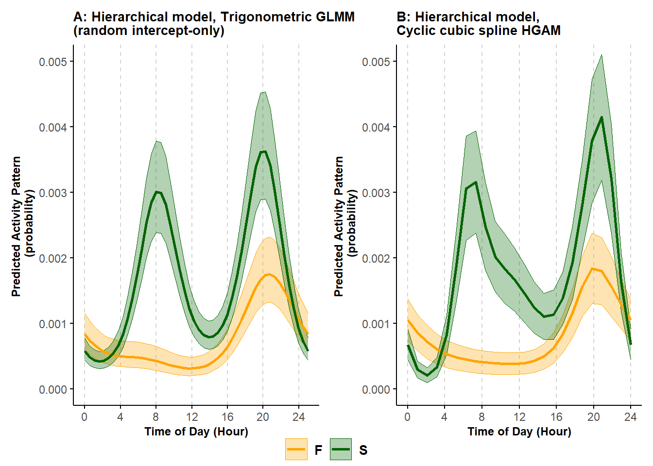
Figure 6.2: Predicted probability of activity of black bears in the spring (S) and fall (F) using a random intercept-only trigonometric hierarchical model (A) and a cyclic cubic spline hierarhical model (B); shading corresponds to 95% confidence intervals.
The patterns estimated by the cyclic cubic spline model closely matches that returned by the random intercept-only trigonometric model, though the curve is slightly more irregular.
Model selection: As done for the trigonometric models, we can use AIC to test the importance of the variable Season by comparing models with and without terms involving the covariate of interest.
# Without general smoother for Time, no covariate effect
mod_cycl1_no_cov <- bam(cbind(success, failure) ~
                          s(Site, bs="re"),
                        knots = list(Time=c(0,23)),
                        family = "binomial",
                        data = occasions_cbind
                        )


AIC(mod_cycl1, mod_cycl1_no_cov)
## df AIC
## mod_cycl1 98.46857 4441.474
## mod_cycl1_no_cov 83.49616 4936.451## [1] 494.977Importantly, (generalized) LRTs should be viewed with some caution. For example, Pedersen et al. (2019) suggest there is insufficient theory to support their use, and S. N. Wood (2017b) note that p-values tend to be too small (usually half of what they should be). Thus, whenever possible, we recommend careful a priori choice of modeling structures based on the desired inference and the characteristics of the data.
We can extend the previous model structure to accommodate site-to-site variability in timing of activity by adding a smoother for Time that depends on Site. We also add a global smoother for Time that shrinks the site-specific estimates towards a common curve. This structure mimics a trigonometric random intercept and random slope model and allows the site-specific activity curves to vary not only in their intercept but also in their shape.
# 'Random intercept and slope'
mod_cycl2 <- bam(cbind(success, failure) ~
                   Season +
                   s(Time, bs = "cc", k = 12) + # global smoother
                   s(Time, bs = "cc", k = 12, by = Site, m = 1) +
                   s(Time, bs = "cc", k = 12, by = Season, m = 1) +
                   s(Site, bs="re"),
                 knots = list(Time=c(0,23)),
                 family = "binomial",
                 data = occasions_cbind
                 )
#summary(mod_cycl2)
AIC(mod_cycl1) - AIC(mod_cycl2)
## [1] 8.390475This model is more supported than the previous one. Plotting some of the estimated site-specific curves shows how the activity patterns can vary greatly among sites.
# Predict site-specific activity patterns
newdat <- with(occasions_cbind,
               expand.grid(Time = seq(min(Time), max(Time), 1),
                           Season = levels(Season),
                           Site =  unique(occasions_cbind$Site)
                           )
               )


cycl_pred1 <- predict.bam(mod_cycl1,
                          newdata = newdat,
                          exclude = NULL,
                          se.fit = TRUE,
                          type = "response"
                          )

cycl_pred1 <- cbind(newdat,
                    fit=cycl_pred1$fit,
                    se.fit=cycl_pred1$se.fit,
                    Model = "Random intercept-only"
                    )

cycl_pred2 <- predict.bam(mod_cycl2,
                          newdata = newdat,
                          exclude = NULL,
                          se.fit = TRUE,
                          type = "response"
                          )

cycl_pred2 <- cbind(newdat,
                    fit=cycl_pred2$fit,
                    se.fit=cycl_pred2$se.fit,
                    Model = "Random intercept and slope"
                    )

cycl_pred <- rbind(cycl_pred1, cycl_pred2)
selected_sites <- c("2A", "2B", "3B", "4D","7B", "14B", "14C", "15A", "15E", "18C")
pl_cycl <- cycl_pred %>% filter(Site %in% selected_sites) %>%
mutate(Season2 = ifelse(Season == "F", "Fall", "Spring")) %>%
ggplot(., aes(Time, fit, group = Site)) +
geom_line(aes(color = Site, group = Site), size = 1) +
labs(x = "Time of Day (Hour)", y = "Predicted Activity Pattern \n (probability)", title = "Cyclic cubic spline HGAMs")+
theme_minimal()+
theme(legend.position = "bottom",
legend.title = element_blank(),
legend.text = element_text(size=10,face="bold"),
legend.margin=margin(0,0,0,0),
legend.box.margin=margin(-5,-10,-10,-10),
plot.title = element_text(size=10,face="bold"),
axis.line = element_line(colour = 'black', linetype = 'solid'),
axis.ticks = element_line(colour = 'black', linetype = 'solid'),
axis.title = element_text(size=9,face="bold"),
panel.grid.minor.y = element_blank(),
panel.grid.major.y = element_blank(),
panel.grid.major.x = element_line(colour = 'lightgrey', linetype = 'dashed', linewidth=0.5),
panel.grid.minor.x = element_blank(),
strip.text = element_text(size = 9, colour = "black", face = "bold", hjust = 0),
plot.margin = margin(0.1,0.1,0.5,0.1, "cm")
) +
scale_x_continuous(breaks=seq(0,max(cycl_pred$Time),length.out=7), labels=seq(0,24,4)) +
facet_grid(Season2~Model)
pl_cycl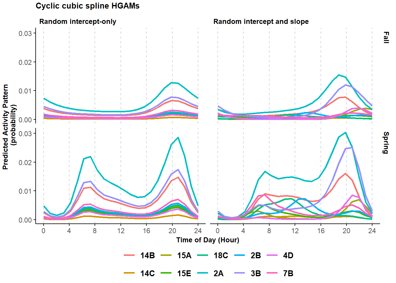
Figure 6.3: Predicted probability of activity of black bears across a select group of sites using a cyclic cubic spline model with a structured resembling a trigonometric random intercept-only (left column) and random intercept and slope (right column) model.
6.2 Continuous covariates
We use the same data to illustrate how hierarchical models can be used to quantify effects of continuous covariates. Specifically, we explore how bear diel activity changes in response to anthropogenic modifications of the landscape quantified through the Global Human Modification index (GHM; Kennedy and Kiesecker (2020); Kennedy and Kiesecker (2019)), a continuous measure of human modification of terrestrial landscapes that ranges between 0 and 1. A histogram of the values of GHM at the different sites indicates that the level of human-driven landscape modification is relatively low in the study area with most sites having a GHM value lower than 0.10.
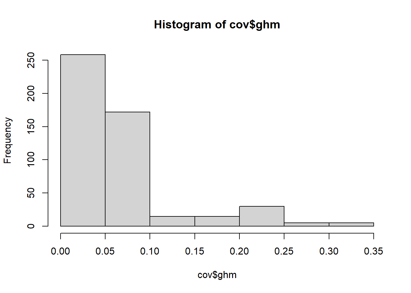
Figure 6.4: Frequency of observed global human modification index (GHM) values across camera sites.
We link the GHM values available in the cov object to the occasion dataframe created at the beginning of this tutorial, and then proceed with arranging the data in the format required to run the hierarchical model as we have done in other examples. This time though, we also add GHM as an additional grouping level.
# Add ghm info
occasions <- left_join(occasions,
                       cov %>% select(Session, Site, ghm)) %>%
  mutate(ghm = round(ghm, digits = 3))
## Joining with `by = join_by(Session, Site)`##
## 0 1
## 0.015 9397 35
## 0.017 15332 28
## 0.018 7849 47
## 0.02 5972 4
## 0.021 4264 8
## 0.022 13961 31occasions$Site <- as.factor(occasions$Site)
# format data for cbind(success, failure)
occasions_cbind <- occasions %>%
group_by(Site, Time, ghm) %>%
summarize(success = sum(capt),
failure = n() - success)## `summarise()` has grouped output by 'Site', 'Time'. You can override using the `.groups` argument.We can now apply either trigonometric GLMMs or HGAMs to the data. As an example, we report a trigonometric random intercept-only model and a cyclic cubic spline HGAM without a site-specific smoother.
# random intercept-only trigonometric GLMM
mod_trig_cont <- mixed_model(fixed = cbind(success, failure) ~ cos(2 * pi * Time/24) * ghm + sin(2 * pi * Time/24) * ghm +
                                                               sin(2 * pi * Time/12) * ghm + cos(2 * pi * Time/12) * ghm,
                             random = ~  1  |   Site,
                             data = occasions_cbind,
                             family = binomial(),
                             iter_EM = 0
                             )
summary(mod_trig_cont)
##
## Call:
## mixed_model(fixed = cbind(success, failure) ~ cos(2 * pi * Time/24) *
## ghm + sin(2 * pi * Time/24) * ghm + sin(2 * pi * Time/12) *
## ghm + cos(2 * pi * Time/12) * ghm, random = ~1 | Site, data = occasions_cbind,
## family = binomial(), iter_EM = 0)
##
## Data Descriptives:
## Number of Observations: 2784
## Number of Groups: 100
##
## Model:
## family: binomial
## link: logit
##
## Fit statistics:
## log.Lik AIC BIC
## -1907.898 3837.795 3866.452
##
## Random effects covariance matrix:
## StdDev
## (Intercept) 0.8716829
##
## Fixed effects:
## Estimate Std.Err z-value p-value
## (Intercept) -6.5825 0.1437 -45.8218 < 1e-04
## cos(2 * pi * Time/24) -0.0752 0.0789 -0.9535 0.34036
## ghm -2.8516 1.5657 -1.8214 0.06855
## sin(2 * pi * Time/24) -0.3062 0.0625 -4.8980 < 1e-04
## sin(2 * pi * Time/12) -0.4642 0.0710 -6.5403 < 1e-04
## cos(2 * pi * Time/12) -0.4561 0.0705 -6.4672 < 1e-04
## cos(2 * pi * Time/24):ghm 0.1742 0.9703 0.1796 0.85750
## ghm:sin(2 * pi * Time/24) 0.8375 0.7415 1.1294 0.25872
## ghm:sin(2 * pi * Time/12) -0.9825 0.8686 -1.1311 0.25802
## ghm:cos(2 * pi * Time/12) -0.6938 0.8599 -0.8068 0.41979
##
## Integration:
## method: adaptive Gauss-Hermite quadrature rule
## quadrature points: 11
##
## Optimization:
## method: quasi-Newton
## converged: TRUE# cyclic cubic spline HGAM without common smoother for Time
mod_cycl1_cont <- bam(cbind(success, failure) ~ ghm +
s(Time, bs = "cc", k = 12, by = ghm, m = 1) +
s(Site, bs="re"),
knots = list(Time=c(0,23)),
family = "binomial",
data = occasions_cbind
)
summary(mod_cycl1_cont)##
## Family: binomial
## Link function: logit
##
## Formula:
## cbind(success, failure) ~ ghm + s(Time, bs = "cc", k = 12, by = ghm,
## m = 1) + s(Site, bs = "re")
##
## Parametric coefficients:
## Estimate Std. Error z value Pr(>|z|)
## (Intercept) -6.2804 0.1353 -46.427 < 2e-16 ***
## ghm -5.8321 1.5420 -3.782 0.000155 ***
## ---
## Signif. codes: 0 '***' 0.001 '**' 0.01 '*' 0.05 '.' 0.1 ' ' 1
##
## Approximate significance of smooth terms:
## edf Ref.df Chi.sq p-value
## s(Time):ghm 7.908 9.079 143.1 <2e-16 ***
## s(Site) 80.847 99.000 603.9 <2e-16 ***
## ---
## Signif. codes: 0 '***' 0.001 '**' 0.01 '*' 0.05 '.' 0.1 ' ' 1
##
## Rank: 112/113
## R-sq.(adj) = 0.243 Deviance explained = 30.7%
## fREML = 4135.1 Scale est. = 1 n = 2784To facilitate understanding, we compare the model-based estimates of activity visually for different quantiles (0.025, 0.5 and 0.975) of the GHM covariate.
# create a new dataset for the estimates
newdat <- with(occasions_cbind,
               expand.grid(Time = seq(min(Time), 24, length.out = 48),
                           ghm = quantile(ghm, probs = c(0.025, 0.5, 0.975)),
                           Site = "7B" # Site does not matter
                           )
               ) %>%
  mutate(ghm_ft = as.factor(ghm),
         ghm_ft = fct_recode(ghm_ft,
                              "Low GHM" = levels(ghm_ft)[1],
                              "Intermediate GHM" = levels(ghm_ft)[2],
                              "High GHM" = levels(ghm_ft)[3])
         )

# trigonometric estimates
cond_eff_cont <- effectPlotData(mod_trig_cont, newdat, marginal = FALSE) %>%
  mutate(pred = plogis(pred),
         low = plogis(low),
         upp = plogis(upp),
         Model = "Trig GLMM"
         )

# cyclic cubic spline estimates
cycl_pred1_cont <- predict.bam(mod_cycl1_cont,
                               newdata = newdat,
                               exclude = "s(Site)",
                               se.fit = TRUE,
                               type = "response"
                               )

cycl_pred1_cont <- cbind(newdat,
                         pred = cycl_pred1_cont$fit,
                         low = cycl_pred1_cont$fit - 1.95*cycl_pred1_cont$se.fit,
                         upp = cycl_pred1_cont$fit + 1.95*cycl_pred1_cont$se.fit,
                         Model = "CC spline HGAM"
                         )

# bring together the estimates based on the two approaches
pred_cont <- rbind(cond_eff_cont, cycl_pred1_cont)
# plot results
ggplot(pred_cont, aes(Time, pred)) +
geom_ribbon(aes(ymin = low, ymax = upp, color = ghm_ft, fill = ghm_ft), alpha = 0.3, linewidth = 0.25) +
geom_line(aes(color = ghm_ft), linewidth = 1) +
scale_color_viridis_d() +
scale_fill_viridis_d() +
labs(x = "Time of Day (Hour)", y = "Predicted Activity Pattern \n (probability)")+
#coord_cartesian(ylim = c(0, 0.005)) +
theme_minimal()+
theme(legend.position = "none",
legend.title = element_blank(),
legend.text = element_text(size=10,face="bold"),
legend.margin=margin(0,0,0,0),
legend.box.margin=margin(-5,-10,-10,-10),
plot.title = element_text(size=10,face="bold"),
axis.line = element_line(colour = 'black', linetype = 'solid'),
axis.ticks = element_line(colour = 'black', linetype = 'solid'),
axis.title = element_text(size=9,face="bold"),
panel.grid.minor.y = element_blank(),
panel.grid.major.y = element_blank(),
panel.grid.major.x = element_line(colour = 'lightgrey', linetype = 'dashed', linewidth=0.5),
panel.grid.minor.x = element_blank(),
strip.text = element_text(size = 9, colour = "black", face = "bold", hjust = 0)
) +
scale_x_continuous(breaks=seq(0,23,length.out=7), labels=seq(0,24,4)) +
facet_grid(Model~ghm_ft)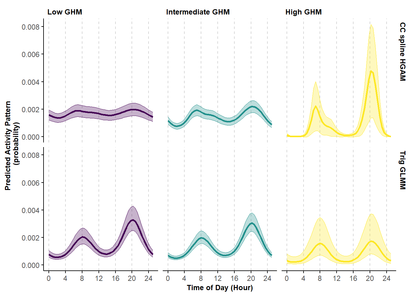
Figure 6.5: Predicted probability of activity by black bears varying by levels of the continuous covariate global human modification index (GHM) using a cyclic cubic spline hierarhical model (first row) and trigonometric hierarhical model (second row).
The estimates based on the cyclic cubic spline HGAM show a clear progression in the shape of black bears’ activity pattern, from having an almost cathemeral pattern at low level of GHM to a well-defined bimodal pattern at the high level of GHM. This trend is less evident in the estimates based on trigonometric GLMM.
We can further evaluate evidence for the effect of GHM on activity by comparing these models with their relative null model (i.e. a version of the model without the covariate of interest) using AIC (or LRT for trigonometric GLMMs).
# null random intercept-only trigonometric GLMM
mod_trig_cont_null <- mixed_model(fixed = cbind(success, failure) ~ cos(2 * pi * Time/24) + sin(2 * pi * Time/24) +
                                                                    sin(2 * pi * Time/12) + cos(2 * pi * Time/12),
                                  random = ~  1  |   Site,
                                  data = occasions_cbind,
                                  family = binomial(),
                                  iter_EM = 0
                                  )


# null cyclic cubic spline HGAM without common smoother for Time
mod_cycl1_cont_null <- bam(cbind(success, failure) ~
                             s(Time, bs = "cc", k = 12, m = 1) +
                             s(Site, bs="re"),
                            knots = list(Time=c(0,23)),
                            family = "binomial",
                            data = occasions_cbind
                           )

# Comparing trig GLMMs
AIC(mod_trig_cont, mod_trig_cont_null)
## df AIC
## mod_trig_cont 11 3837.795
## mod_trig_cont_null 6 3833.623## [1] -4.17234## df AIC
## mod_cycl1_cont 91.44899 3825.111
## mod_cycl1_cont_null 91.92963 3709.086## [1] -116.0255We find that there is little support for an effect of GHM on the activity patterns of American black bear, which is perhaps not surprising given the low level of human disturbance at these sites.